A rollout engine and a training engine can load the same checkpoint, read the same token prefix, and still assign different probabilities to the next token. For RL fine-tuning, that numerical gap changes the distribution behind the policy-gradient estimate.
The previous post examined exploration through GRPO, DAPO and GSPO. Here I focus on an implementation detail beneath those objectives: the choice between BF16 and FP16. BF16 offers a wide numerical range; FP16 allocates more bits to precision. Qi et al.’s Defeating the Training-Inference Mismatch via FP16 found that this difference can substantially reduce rollout–trainer mismatch in their RL experiments.
I use a small NumPy model to examine one possible mechanism. Two implementations share weights and rounding points but accumulate matrix products differently. The experiment shows how rounding can turn small execution differences into persistent probability differences. It also illustrates an exact fact about likelihood ratios: on samples from the rollout policy, the trainer’s log-probability has a negative average offset equal to a KL divergence. Over a long response, that offset can matter as much as the random variation around it.
The toy has no attention, reward, or policy updates. It is a controlled numerical experiment; its error ratios are measurements of this configuration.
What the formats trade
FP16 and BF16 each use one sign bit. They allocate the remaining bits differently:
| Format | Exponent bits | Fraction bits | Largest finite value | Smallest positive normal | Spacing above 1 |
|---|---|---|---|---|---|
| FP32 | 8 | 23 | ≈ 3.40 × 10³⁸ | ≈ 1.18 × 10⁻³⁸ | 2⁻²³ |
| FP16 | 5 | 10 | 65,504 | ≈ 6.10 × 10⁻⁵ | 2⁻¹⁰ |
| BF16 | 8 | 7 | ≈ 3.39 × 10³⁸ | ≈ 1.18 × 10⁻³⁸ | 2⁻⁷ |
The fraction-bit counts exclude the implicit leading bit of a normal number. For a positive normal value \(x\), away from the upper range boundary, the local spacing is
\[ \operatorname{ulp}(x)=2^{\lfloor\log_2 x\rfloor-m}, \]
where \(m\) is the number of fraction bits. Within each power-of-two interval, the relative spacing lies between \(2^{-(m+1)}\) and \(2^{-m}\). Where both formats represent normal numbers, FP16’s grid is eight times finer than BF16’s. That is a statement about representable values, not an eightfold guarantee for a network’s output error.
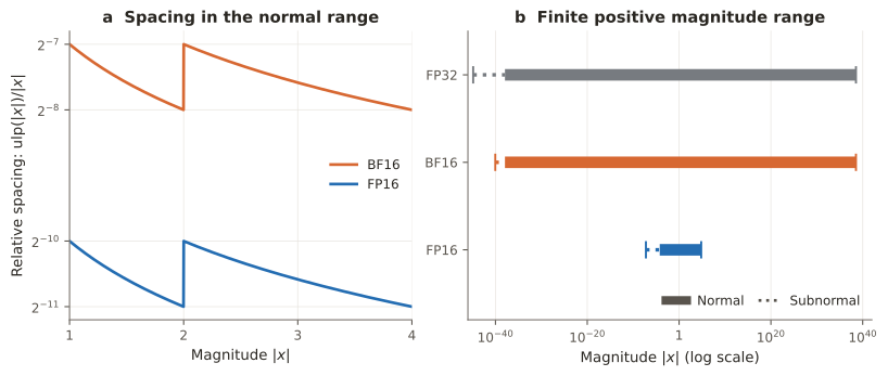
This trade explains BF16’s appeal for large-model training. Micikevicius et al. established an FP16 mixed-precision recipe using FP32 master weights and loss scaling to preserve small gradients. Kalamkar et al. showed that BF16’s FP32-like exponent range made mixed-precision training practical across several workloads without the same need for loss scaling. BF16 greatly reduces range-related difficulties, though it does not make overflow, underflow, or NaN impossible.
For RL on an existing checkpoint, the question is whether FP16’s narrower range is acceptable in exchange for finer resolution. A pretrained model does not automatically satisfy that condition: its activations were never required to fit within FP16’s range, and they can change during fine-tuning.
Same weights, different policies
It helps to distinguish three policies for a prompt \(x\):
- \(\mu_{\mathrm{old}}\): the distribution that actually sampled the response;
- \(\pi_{\mathrm{old}}\): the training engine evaluated at those same old weights;
- \(\pi_\theta\): the training engine at the current weights.
The full response-level importance ratio factors into two terms:
\[ \frac{\pi_\theta(y\mid x)}{\mu_{\mathrm{old}}(y\mid x)} = \underbrace{\frac{\pi_\theta(y\mid x)}{\pi_{\mathrm{old}}(y\mid x)}}_{\text{policy update}} \underbrace{\frac{\pi_{\mathrm{old}}(y\mid x)}{\mu_{\mathrm{old}}(y\mid x)}}_{\text{engine mismatch}}. \]
Even before a gradient update, the second term can differ from one. Recomputing old log-probabilities with the trainer removes this term from a trainer-to-trainer ratio, but does not change the distribution that generated the data.
For the expected-reward objective, importance weighting gives the usual identity
\[ \nabla_\theta J(\theta) = \mathbb E_{y\sim\mu_{\mathrm{old}}} \left[ \frac{\pi_\theta(y)}{\mu_{\mathrm{old}}(y)} \bigl(R(y)-b(x)\bigr) \nabla_\theta\log\pi_\theta(y) \right], \]
with a prompt-dependent baseline \(b(x)\) and the prompt suppressed elsewhere. This assumes that the behavior distribution covers the target’s support and that the denominator is the actual sampling probability. Temperature, top-\(p\), token masks, and stopping rules must be accounted for. Clipping and group-normalized advantages introduce additional choices beyond this identity.
The engine gap is well documented. Yao et al. described its off-policy consequences and a token-level truncated importance-sampling correction. Liu et al. examined sequence-level corrections and masking. MiniMax-M1, §3.2, traced a damaging mismatch to large activations in the LM output head and improved consistency by using FP32 there. The Qwen team’s analysis also discusses kernel differences and MoE routing.
Qi et al. tested another lever: FP16. Their offline analysis used DeepSeek-R1-Distill-Qwen-1.5B with temperature 1 and no top-\(p\), so the probabilities were directly comparable. Figure 2 reports sequence KL values of 7.64 for BF16 and 0.32 for FP16, a ratio of about 24. In a separate 1.5B sanity test, FP16 importance-weighted policy gradient outperformed the BF16 baselines. Further experiments covered larger dense models, MoE, and LoRA under different algorithmic settings. These results motivate examining precision; they do not establish a universal multiplier. See the offline analysis and the training experiments for their separate settings.
A controlled numerical experiment
The toy is a recurrent residual MLP: four blocks, width 256, SiLU activations, RMSNorm, and an 8,192-token vocabulary. Its recurrence carries a state between tokens. The recurrent matrix is initialized with a \(0.9/\sqrt{256}\) scale; this is an initialization choice, not a guarantee that the nonlinear system is contractive. The output scale is 14, producing mean next-token entropy near 0.55 nats in these runs. This creates confident distributions without modeling the semantics of reasoning.
For each format, both engines use the same cast weights:
- The rollout engine computes matrix products in 64-element split-K chunks and adds their FP32 partial sums sequentially.
- The trainer engine uses a single FP32 BLAS call for each matrix product.
Both apply the same storage-rounding operations. BF16 is emulated with round-to-nearest-even; FP16 uses NumPy’s float16. The scripts specify the rounding points explicitly. This emulates storage precision and a reduction-order difference, rather than executing GPU Tensor Core kernels.
For measurement, both engines’ logits are converted to normalized FP64 log-probabilities. Sampling also uses FP64. This avoids letting the diagnostic softmax or cumulative sampler dominate a very small mismatch. All model matrix products remain FP32, with the selected format’s rounding applied as specified. A separate small-model control gives exactly zero sampled mismatch, conditional KL, and state discrepancy in all four conditions when both engines use identical accumulation.
Each condition generates 128 responses of 2,048 tokens for each of three sampling seeds: 384 responses in total, with one fixed model initialization. Every sampled token is scored by both engines on the same token prefix. Across formats, the weights after casting and the sampled prefixes can differ. The confidence intervals below resample whole responses and describe sampling uncertainty for this model and environment.
Rounding can erase a difference—or enlarge it
Start with one matrix multiplication, before recurrence or depth can amplify anything:
| Output format | Elements that differ | Median relative gap among differing elements | Relative Frobenius norm difference |
|---|---|---|---|
| FP32 | 90% | 2.9 × 10⁻⁷ | 3.01 × 10⁻⁷ |
| FP16 | 0.142% | 6.71 × 10⁻⁴ | 1.23 × 10⁻⁵ |
| BF16 | 0.00827% | 5.41 × 10⁻³ | 2.19 × 10⁻⁵ |
Most small differences between the two FP32 computations disappear when both results round to the same 16-bit value. A minority straddle a rounding boundary and become a full-ulp difference. A coarser grid can make these events less frequent but larger when they occur. Consequently, the norm difference after one operation does not simply scale with the ratio of fraction-bit counts.
Subsequent layers transform those perturbations. They may attenuate them, preserve them, or amplify them, depending on the weights, activations, normalization, and rounding boundaries. In this toy, the relative state discrepancy settles near the normal-range spacing of each 16-bit format after the initial transient.
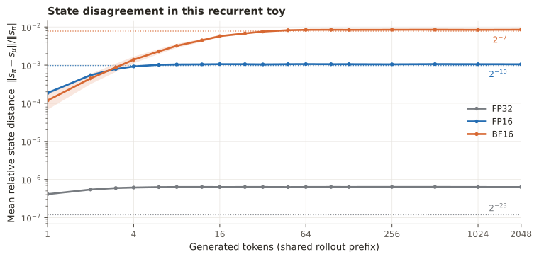
The mechanism is therefore conditional: a small execution difference can survive rounding and propagate through the model. Its eventual size remains a property of the model and the execution path, as well as the format.
From states to token probabilities
Write \(\mu\) and \(\pi\) for the rollout and trainer distributions at the same weights, and define
\[ d_t=\log\pi(y_t\mid y_{<t})-\log\mu(y_t\mid y_{<t}), \qquad y_t\sim\mu(\cdot\mid y_{<t}). \]
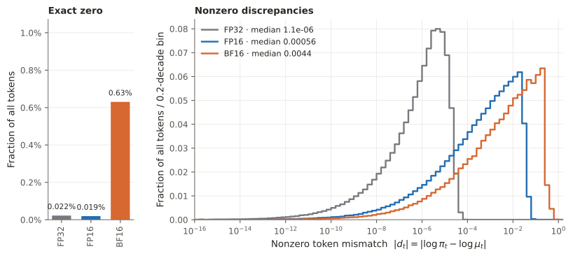
In these runs, the mean absolute token mismatch is 8 times larger in BF16 than in FP16. The table also reports a different quantity: conditional KL, summed over the entire vocabulary at each visited prefix. Computing it directly avoids the extra variance of estimating a small KL from only the sampled token’s log-ratio.
| Format | Mean absolute token mismatch | Conditional KL per token | Sequence RMS at 2,048 |
|---|---|---|---|
| FP32 | 4.14 × 10⁻⁶ | 3.16 × 10⁻¹¹ [3.15, 3.17] × 10⁻¹¹ |
3.49 × 10⁻⁴ [3.25, 3.71] × 10⁻⁴ |
| FP16 | 4.88 × 10⁻³ | 5.15 × 10⁻⁵ [5.13, 5.16] × 10⁻⁵ |
0.469 [0.435, 0.5] |
| BF16 | 0.039 | 3.28 × 10⁻³ [3.27, 3.29] × 10⁻³ |
7.57 [7.23, 7.92] |
| BF16 + FP32 head | 0.032 | 1.89 × 10⁻³ [1.89, 1.9] × 10⁻³ |
4.69 [4.42, 4.97] |
The intervals are 95% response-bootstrap intervals. The sequence RMS is \(\sqrt{E[S_T^2]}\), where \(S_T=\sum_{t=1}^T d_t\), at \(T=2{,}048\). KL, absolute token error, and sequence RMS answer different questions; their ratios need not agree.
Low-probability sampled tokens show larger log-probability changes in this experiment. The relevant local sensitivity is
\[ \delta\log p_y=\delta z_y-\sum_v p_v\,\delta z_v. \]
A highly confident prediction tends to cancel a perturbation shared by its selected logit and the probability-weighted average. A low-probability token has less of that protection. This explains a possible sensitivity pattern; low probability alone does not establish that a token carries a more useful learning signal.
Why sequence mismatch develops a drift
For a fixed prefix, with normalized distributions and the support condition above,
\[ \mathbb E_{y_t\sim\mu}[e^{d_t}\mid y_{<t}]=1, \qquad \mathbb E_{y_t\sim\mu}[d_t\mid y_{<t}] =-\mathrm{KL}\bigl(\mu_t\|\pi_t\bigr). \]
This is exact. The mean log-ratio is nonpositive even when both implementations use the same weights. For a fixed horizon \(T\), averaging over rollout prefixes gives
\[ \mathbb E_\mu[S_T] =-\sum_{t=1}^T \mathbb E_{Y_{<t}\sim\mu} \left[\mathrm{KL}\bigl(\mu_t(\cdot\mid Y_{<t})\|\pi_t(\cdot\mid Y_{<t})\bigr)\right]. \]
No independence assumption is needed for that drift identity. Variance requires more care:
\[ \operatorname{Var}(S_T) =\sum_t\operatorname{Var}(d_t) +2\sum_{s<t}\operatorname{Cov}(d_s,d_t). \]
Suppose the average per-token KL is approximately constant at \(\kappa\), the token log-ratio variance is approximately \(\sigma^2\), and the cumulative covariance is small. Then
\[ \mathbb E[S_T]\approx-T\kappa, \qquad \operatorname{SD}(S_T)\approx\sqrt{T}\,\sigma, \qquad \operatorname{RMS}(S_T)\approx\sqrt{T\sigma^2+T^2\kappa^2}. \]
The mean grows in magnitude with \(T\); the standard deviation grows like \(\sqrt T\) under this approximation. Figure 4 plots them separately, so their agreement with the approximation can be inspected rather than inferred from a small lag-1 correlation.
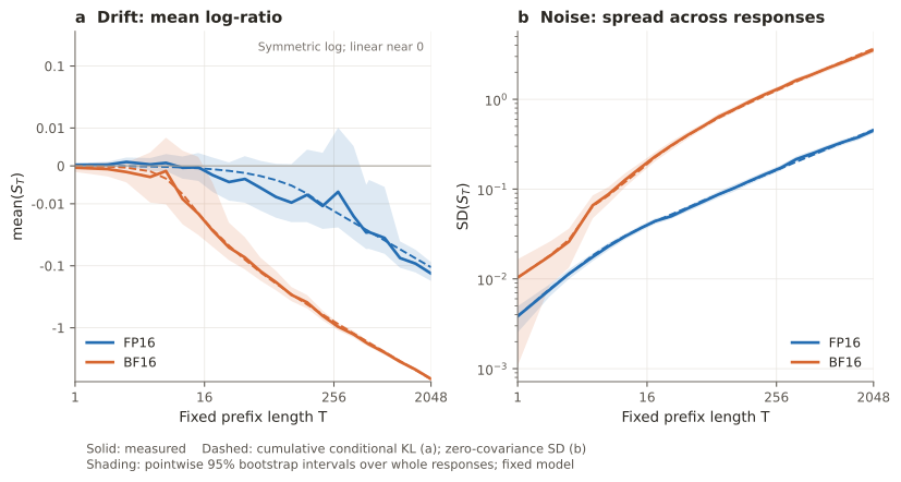
At 2,048 tokens, the measured sequence variance divided by the sum of the individual token variances is 0.96 for FP16 and 0.93 for BF16. The omitted covariance is modest here, although that need not hold in a different model.
For small log-ratio perturbations, the cumulant expansion of \(\log E[e^{d_t}]=0\) gives \(\kappa\approx\sigma^2/2\), provided higher-order terms are negligible. This yields the familiar approximation
\[ \operatorname{RMS}(S_T) \approx\sqrt{T\sigma^2+(T\sigma^2/2)^2}. \]
It explains how an eightfold change in the token noise scale could have a larger effect on long-sequence RMS: the noise term scales with \(\sigma\), while the approximate drift scales with \(\sigma^2\). In this experiment the measured BF16/FP16 sequence RMS ratio is 16.2 at 2,048 tokens, and the directly computed per-token KL ratio is 63.8. These are results for the toy, not an explanation of Qi et al.’s particular 24× sequence-KL measurement. Their metric and experimental distribution differ.
The distinction also matters statistically. Estimating KL as \(-\operatorname{mean}(d_t)\) is valid under the stated conditions but can be noisy when KL is small. The released analysis reports that estimate, a control-variate estimate \(\operatorname{mean}(e^{d_t}-1-d_t)\), and the direct conditional KL. The article uses the direct calculation for its KL claims.
What this suggests for RL objectives
Reducing engine mismatch can make off-policy correction easier. The exact effect on a gradient estimator depends on rewards, score functions, tail behavior, and the correction rule. The negative mean of \(d_t\) is a KL identity; it does not imply that gradient bias or gradient variance scales as \(\sigma^2\). Even the variance of the importance weight is a different divergence: \(\operatorname{Var}_\mu(\pi/\mu)=\chi^2(\pi\|\mu)\) when the second moment exists.
Sequence ratios combine all token log-ratios, so their distribution can change substantially with length. A token-level correction does not generally recover the full sequence change of measure. Truncation and masking then make different tradeoffs: some cap or reject only large ratios, while other rules use two-sided intervals. Negative log-ratio drift alone does not tell us how often any particular rule activates.
A note on GSPO. GSPO, Eq. 7 and §5.4, uses a length-normalized sequence ratio and discusses using rollout-engine likelihoods directly. If those likelihoods supply the denominator, then at the same checkpoint the mismatch contribution satisfies
\[ \log s(y)=\frac{S_T}{T}, \qquad E[\log s]\approx-\kappa, \qquad \operatorname{SD}(\log s)\approx\frac{\sigma}{\sqrt T}. \]
Length normalization reduces fluctuations under the weak-dependence approximation but leaves the mean log-ratio offset. In this toy the BF16 offset is larger than the lower clipping width \(3\times10^{-4}\) used in the cited GSPO experiment; its upper width is \(4\times10^{-4}\). This is a useful diagnostic comparison, not a test of GSPO. The clipped surrogate depends on the advantage sign: a low ratio enters the clipped branch for negative advantages, while a high ratio does so for positive advantages. The toy has neither advantages nor policy updates, and a current-policy ratio would also include the genuine weight-update term.
An FP32 LM head is another useful diagnostic. In the head ablation, its weights and output logits stay FP32 while the rest of the model uses BF16. Conditional KL falls by 42.3%, but remains 36.8 times the FP16 value. This shows that, in this toy, disagreement has already developed below the head. MiniMax’s real-model result should be read in its own context: the team located the dominant problem in its output layer and fixed that layer.
Choosing what to measure—and what to change
A precision change should be evaluated at fixed weights before interpreting a training curve. A practical comparison has four parts:
- Align the probability definitions. Score the same token prefixes, using the same checkpoint, temperature, masks, and stopping conventions. Separate engine mismatch from changes introduced by policy updates.
- Measure both token and sequence behavior. Report conditional KL where feasible, distributions of sampled-token log-ratios, and sequence means and spreads at fixed prefix lengths. Include uncertainty across responses. Low-probability-token slices can reveal errors that an overall average hides.
- Check FP16’s range. Its maximum finite value is 65,504. Its smallest positive subnormal is \(2^{-24}\approx5.96\times10^{-8}\); rounding to zero and hardware flush-to-zero behavior require separate treatment. FP32 master weights and dynamic loss scaling can preserve small updates and gradients, but loss scaling cannot repair a forward activation that has already overflowed.
- Recheck during optimization. Weights, activations, routing, and response lengths evolve. A favorable fixed-checkpoint result does not guarantee a stable training run.
The last point has direct evidence. Zhang et al., §4.4, observed collapse under FP16 as well as BF16 in their experiments, and stabilized the FP16 run with their learning-rate schedule. That result limits any claim that changing the format is sufficient.
When studying length, use a fixed-prefix design with an explicit EOS convention. Bucketing naturally terminated responses by their final length conditions on a stopping event; the fixed-\(T\) drift formula cannot be applied to those buckets without accounting for that selection.
There are also direct engineering remedies. He and Thinking Machines Lab demonstrated batch-invariant execution and aligned sampling/training stacks with zero measured mismatch. The Miles alignment write-up describes bitwise alignment across SGLang and training backends, alongside algorithmic correction options. MoE routing replay targets another specific source. These approaches address different parts of the system; their throughput and engineering costs need measurement on the intended workload.
FP16 is therefore a useful experiment when range permits and engine mismatch is material. The format changes the rounding grid. The resulting policy difference must still be measured, and the need for correction should be judged from that difference and the training objective.
Reproducing the experiment
Download the source, recorded results, and environment metadata. The package includes the four conditions, three sampling seeds, full-vocabulary KL diagnostics, response-bootstrap intervals, and the scripts that produce every table and figure. The README gives one command for a complete rerun and a faster command to regenerate figures from the recorded data.
The recorded run uses Python 3.12.14, NumPy 2.3.5, and Apple Accelerate BLAS on macOS arm64. One model initialization is held fixed throughout. Different BLAS implementations can change small numerical differences and, eventually, sampled trajectories even with the same random seed. The intervals quantify sampling variability for this setup; they do not describe variation across architectures, model initializations, or hardware.
References
- Qi, P., Liu, Z., Zhou, X., Pang, T., Du, C., Lee, W. S., & Lin, M. (2025). Defeating the Training-Inference Mismatch via FP16.
- Yao, F., Liu, L., Zhang, D., Dong, C., Shang, J., & Gao, J. (2025). Your Efficient RL Framework Secretly Brings You Off-Policy RL Training.
- Liu, J., Li, Y., Fu, Y., Wang, J., Liu, Q., & Shen, Y. (2025). When Speed Kills Stability: Demystifying RL Collapse from the Training-Inference Mismatch.
- He, H., & Thinking Machines Lab. (2025). Defeating Nondeterminism in LLM Inference.
- MiniMax. (2025). MiniMax-M1: Scaling Test-Time Compute Efficiently with Lightning Attention.
- Zheng, C., Liu, S., Li, M., et al. (2025). Group Sequence Policy Optimization.
- Zheng, C., Dang, K., Yu, B., et al. (2025). Stabilizing Reinforcement Learning with LLMs: Formulation and Practices.
- Zhang, Y., Li, Y., Liu, J., Xu, J., Li, Z., Liu, Q., & Li, H. (2026). Beyond Precision: Training-Inference Mismatch is an Optimization Problem and Simple LR Scheduling Fixes It.
- Micikevicius, P., Narang, S., Alben, J., et al. (2018). Mixed Precision Training. ICLR 2018.
- Kalamkar, D., Mudigere, D., Mellempudi, N., et al. (2019). A Study of BFLOAT16 for Deep Learning Training.